Risk Assessment in Convolutional Neural Network Text Classification

Our intern Maurizio Sluijmers has recently completed his master’s degree in Econometrics and Mathematical Economics at Tilburg University. For his thesis, he investigated the application of Convolutional Neural Networks in Text Classification with an emphasis on Risk Assessment. This blog post summarizes his findings and provides insights into the broader topics he explored.

Overview of Text Classification and Risk Assessments  

Natural Language Processing (NLP) has always been a foundational element in Artificial Intelligence (AI) research. The primary aim of NLP is to comprehend and interpret human languages effectively. Among the various domains of NLP, text classification is one of the most developed areas. Its goal is to automate the categorization of textual data into one or more predefined categories, thus offering a rapid and cost-effective method to structure textual information. Traditional methods like Logistic Regression and Support Vector Machines can be utilized, but more advanced deep learning techniques such as Convolutional Neural Networks (CNN) have also proven to be effective. The potential of CNNs in text classification was notably highlighted by Kim (2014), leading to their rapid adoption in the field (Sun and Gu, 2017).

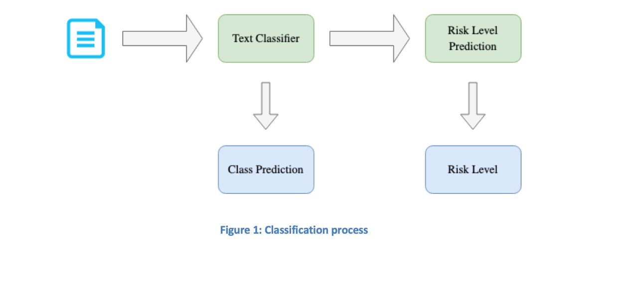
However, a significant drawback in text classification is the uncertainty surrounding the accuracy of the class predictions. This ongoing uncertainty necessitates human intervention for verification. While manual categorization is no longer required, the output from text classifiers still needs to be assessed and adjusted. Reducing this manual verification would be advantageous, hence enhancing the model to provide a confidence level alongside each prediction could be beneficial. This can be accomplished by utilizing the classifier’s results to predict risk levels (RLP). RLP assigns a risk value to each prediction, indicating whether it is high risk or low risk. This improves the classification system’s effectiveness by allowing the model to recognize potential errors, thereby streamlining manual efforts. Class predictions deemed low risk can proceed without further checks, while those classified as high risk require human validation.

The proposed classification workflow is illustrated in Figure 1 below.

Text Classification  

Text classification increasingly plays a pivotal role in businesses, providing efficient insights from textual data and automating various processes. By utilizing text classifiers, tasks historically performed manually can now be automated. For instance, sentiment analysis categorizes user reviews into positive, negative, or neutral sentiments, while product classification assigns products to corresponding categories based on their textual descriptions.

The field of text classification is extensive, with various techniques available to solve classification challenges (Kowsari et al., 2019). This post will examine three distinct approaches to text classification.

Approach 1: TF-IDF Logistic Regression  

TF-IDF logistic regression is a straightforward yet effective classification method that has demonstrated competitive results over the years (Wang et al., 2017). It generates TF-IDF feature vectors from the texts, which are then utilized to classify the information using logistic regression. TF-IDF refers to Term Frequency — Inverse Document Frequency, which gauges the significance of a word in a text by computing a score based on its frequency within that text compared to its frequency across the entire text collection. While the advantage of TF-IDF lies in emphasizing words that convey meaningful information, a notable limitation is that it disregards word order and context, preventing the classifier from capturing semantic nuances.

The logistic regression classifier is trained on these TF-IDF feature vectors and can subsequently make predictions for new texts based on their corresponding feature vectors.

Approach 2: Convolutional Neural Network  

In contrast to the TF-IDF logistic regression, Convolutional Neural Networks (CNNs) factor in word context and relationships in texts. This is achieved through the use of word embeddings.

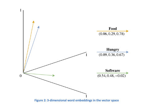
Word embeddings aim to convert human language into a significant numerical format. Each word is represented as a vector, and proximity of these vectors in the vector space indicates semantic connections. A distinct word embedding vector is created for each word in the dataset. For instance, in Figure 2, a simplistic representation of 3-dimensional word embeddings for “food,” “hungry,” and “software” is presented, highlighting that “food” and “hungry” are closely related, while “software” is not. Typically, word embeddings are defined in higher dimensions (often 50, 100, 200, or 300) to enhance the distinction between words.

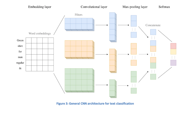
Next, we will examine a specific architecture of CNNs, as outlined in Figure 3. CNNs consist of interconnected layers, commencing with the embedding layer that takes integer-encoded texts as input and initializes either random or pre-trained word embedding weights. These weights are refined during training through updates in each epoch (an epoch signifies a complete cycle through the network). Figure 3 illustrates the word embeddings for the phrase “Green shirt for men regular fit,” with a dimensionality of 5 for visualization purposes.

Following is the convolutional layer, which processes the sequences of word embeddings and creates feature vectors by examining the word embeddings for each text through the use of convolution filters. These filters, which are matrices filled with weights, analyze several consecutive words simultaneously and traverse the text to generate a feature map. This operation is executed for all texts using multiple convolution filters, highlighting diverse relationships between words. Filters may vary in height, affecting how many consecutive words they evaluate in each step. The feature vectors are generated by adding a bias term to the resulting feature maps and applying an activation function (ReLU is the most commonly utilized activation function) to introduce non-linearity that enables the learning of complex relationships.

The pooling layer receives the variable-length feature vectors from the convolutional layer and converts them into fixed-length vectors, discarding less relevant local information.

The final layer of the CNN is the softmax layer. This layer receives fixed-length feature vectors that first proceed through a fully-connected layer, which efficiently learns non-linear combinations of features. The output from this layer consists of numerical values corresponding to each classification. The softmax function is then applied to interpret these numbers as predicted probabilities for each class, with the class showing the highest predicted probability becoming the predicted class from the CNN.

During CNN training, the weights in the embedding, convolutional, and softmax layers are continually updated using the categorical cross-entropy loss function in each epoch. Back-propagation, which is fundamental to neural network training, involves distributing the total loss obtained from forward propagation back through the CNN, allowing for the identification of the loss contribution of each node, leading to weight adjustments that minimize the overall loss.

Approach 3: Soft Voting  

We have now covered two distinct text classification methods—logistic regression and CNN. To enhance the performance of both models, we can combine them into an ensemble text classifier. This can be achieved using a Soft Voting (SV) classifier, which predicts classes by calculating a weighted average of the probabilities derived from both the LR and CNN classifiers. This voting mechanism can help balance the individual weaknesses of the classifiers. To configure the SV text classifier, weights for the predicted probabilities from both the LR and CNN models need to be determined using a separate validation set of texts not employed in training.

Once the weights are established, the soft vote model can calculate the weighted predicted probabilities for each class, with the SV classifier’s predicted class being the one that attains the highest weighted predicted probability.

Risk Level Prediction  

As alluded to earlier, uncertainty exists regarding the accuracy of predictions made by text classifiers. To address this issue, a methodology for evaluating the risk associated with class predictions is necessary. Risk Level Prediction (RLP) offers a risk assessment for each class prediction made by the text classifier, aiming to provide a critical perspective on the reliability of each prediction, which indicates how ‘uncertain’ the model is about its output. Consequently, only predictions with elevated risk levels necessitate manual verification, as these predictions include a greater degree of uncertainty.

Methodology  

In multi-class classification, the class with the highest predicted probability from the text classifier is assigned to the text. The predicted probability may serve as a valuable risk indicator, wherein higher probabilities reflect greater confidence in the prediction’s accuracy. Though the predicted probability of the classified category can indicate risk, incorporating multiple risk indicators may enhance prediction accuracy.

RLP’s foundational concept is to train an additional classifier that utilizes specific risk indicators to determine if a prediction is ‘correct’ or ‘wrong.’ It is essential to allocate training data into two distinct subsets: one for training the text classifier, and the other for the RLP classifier. The process proceeds as follows:

1. The text classifier is trained using the first subset of data.
2. The trained text classifier is then applied to classify texts in the second subset, generating both predicted and true classes. By comparing these predictions, we assess correctness, resulting in a binary outcome serving as the target variable for the RLP classifier. Utilizing risk indicators as input features, this classifier is trained to assess whether new texts’ assigned classes are accurate.

Our objective is to cultivate an RLP classifier capable of accurately discerning the correctness of a text classifier’s class predictions. This allows us to assign corresponding risk levels based on the binary classifier’s results. To achieve this, it is vital to extract indicators that highlight prediction uncertainty. Suitable features may involve the top-k predicted probabilities (i.e., the k highest probabilities), sentence statistics (e.g., text length), class behavior metrics (e.g., class F1-score), etc.

RLP Variants  

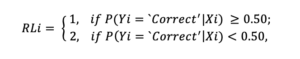
The RLP utilizes a binary classifier that categorizes text classifier output as either ‘correct’ or ‘wrong.’ The binary classifier’s classifications operate on traditional decision boundaries: if the predicted probability exceeds 0.50, it is deemed ‘correct’; otherwise, it is labeled ‘wrong.’ Risk levels are thus assigned based on these probabilities, where a binary classifier’s prediction above 0.50 corresponds to a risk level of 1 (not risky, reliable prediction) and below equates to a risk level of 2 (risky, unreliable prediction). The risk level (RL) for a particular text prediction is determined as illustrated in the photo, with Y representing the binary target variable and X denoting the features.

The RLP variant discussed employs a singular binary classifier for risk level predictions. However, it’s possible to enhance this approach by using two binary classifiers. A straightforward method involves assigning a risk level of 1 when both classifiers predict ‘correct,’ while any other outcome yields a risk level of 2.

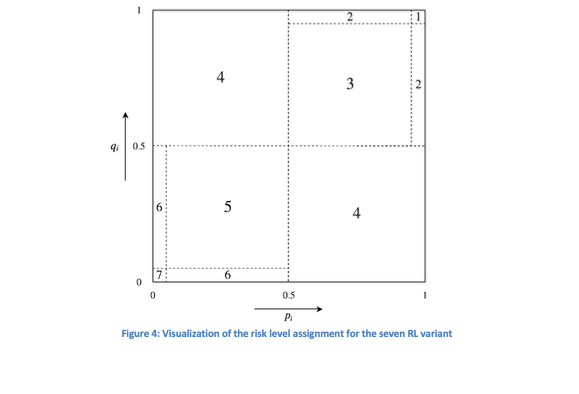
This framework can also be adapted to produce more than two risk levels. For instance, when both classifiers confidently predict ‘correct,’ a low-risk level is assigned; if one classifier predicts ‘correct’ with certainty and the other with less, a moderately risk can be indicated. This reasoning can be extended further to derive various risk levels. An example illustrating seven distinct risk levels from the results of two binary classifiers is illustrated in Figure 4, with pi and qi representing the predicted probabilities of the respective classifiers.

The various RLP variants discussed exemplify different strategies for assigning risk levels, with potential for additional modifications based on unique requirements.

Classification System  

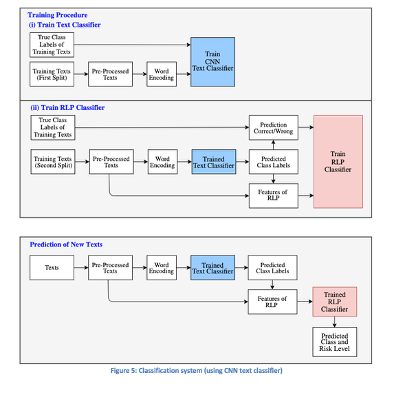
Figure 5 provides a comprehensive overview of the classification system discussed throughout this post. The CNN text classifier is employed for class predictions, beginning with its training on the first portion of the training data, followed by training the RLP’s binary classifier on the second portion. Both the text classifier and the RLP can then be applied to new texts to generate predictions and corresponding risk assessments.

References  

• Kim, Y. (2014). Convolutional Neural Networks for Sentence Classification. Proceedings of the 2014 Conference on Empirical Methods in Natural Language Processing (EMNLP).
• Kowsari, K., Meimandi, K.J., Heidarysafa, M., Mendu, S., Barnes, L. and Brown, D. (2019). Text Classification Algorithms: A survey. Information, 10(4), 150.
• Sun, S. and Gu, X. (2017). Word Embedding Dropout and Variable-Length Convolution Window in Convolutional Neural Network for Sentiment Classification. ICANN 2017 (2), 40–48.
• Wang, Y., Zhou, Z., Jin, S., Liu, D. and Lu, M. (2017). Comparisons and Selections of Features and Classifiers for Short Text Classification. IOP Conference Series: Materials Science and Engineering, 261.
• Wang, Zhou, Jin, Liu, Lu (2017) Comparisons and selections of features and classifiers for short text classification.