Implementing Reinforcement Learning for Order-Pick Routing in Warehouses

Overview of Reinforcement Learning  

Reinforcement Learning (RL) is increasingly relevant in machine learning, with applications ranging from self-driving vehicles to game-playing bots. However, its use in operational challenges remains limited. This article walks through the fundamental principles of Reinforcement Learning and demonstrates its effectiveness in addressing a basic order-pick routing scenario within a warehouse using Python.

RL is versatile in its applicability and, as stated by Bhatt [?]: “Reinforcement Learning is a machine learning strategy that allows an agent to learn from its interactions with the environment via trial and error, utilizing feedback from its own actions.” Unlike supervised learning, RL is unsupervised, which means it does not require labeled input/output data.

In RL, a problem is typically represented as a Markov Decision Process (MDP) comprising:

• Environment: The surrounding world where the agent functions.
• State: The current condition of the environment, represented as a set S.
• Action: Decisions made by the agent that influence the environment, denoted as set A. Each state s ∈ S may have a unique set of allowable actions indicated as A(s).
• Reward: The feedback received from the environment, with the reward for transitioning from state s to s′ using action a symbolized as ra(s, s′).
• State-action-transition probability: The likelihood of moving from state s to state s′ given action a, represented as p(s′ | s, a). This creates a comprehensive set of probabilities denoted by P.

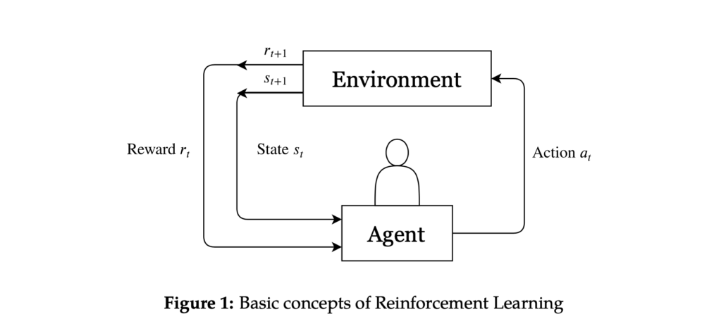
These elements are depicted in figure 1. At each discrete timestep t, the agent observes its state st and performs an action at from the available actions. Following this action, the environment updates to a new state st+1, and the agent receives a reward rt+1 resulting from the transition (st, at, st+1). The primary objective for the agent is to maximize future rewards by learning from the consequences of its actions in the environment. Consequently, the agent must balance between immediate and long-term rewards at each timestep.

Owing to its broad applicability, Reinforcement Learning can tackle numerous challenges. RL is often utilized for developing AI in computer games like Pac-Man, backgammon, and AlphaGo, as well as for creating software for autonomous vehicles.

Framing Order-Pick Routing as a RL Problem  

Now that we have grasped the key concepts of RL, we should explore how to frame our order-pick routing challenge within these principles.

The order-picking task in a warehouse resembles a variant of the classic Traveling Salesman Problem (TSP), which inquires: “Given a list of locations and the distances between each, what is the shortest route that visits each location before returning to the starting point?” In the context of order-pick routing, this question can be rephrased: “Given a list of pick locations and the distances between them, what is the most efficient route to visit each pick location and return to the I/O point?” The TSP is a well-researched subject within combinatorial optimization, with numerous heuristics established for solving it. We can outline the warehouse order-pick routing as an MDP:

An agent (a worker with a cart) moves through the warehouse (the environment) to collect items from designated pick nodes. At each timestep t, the agent must choose which node to visit next, marking it from unvisited to visited (the state). The objective is to determine the most efficient order for visiting these nodes, maximizing the negative total distance (the reward). The fundamental components of this MDP are as follows:

• State: Represents the environment of the warehouse, containing the current node and a list of unvisited nodes. st encompasses the current pick location and remaining nodes to be visited.
• Action: A finite set of choices A involving the next node to visit. This set can either be common across all states s ∈ S or reduce over time. Once all nodes are visited at timestep t, the only action left is to return to the I/O point.
• Reward: Environmental feedback; the reward for transitioning from state s to s′ after taking action a is typically the negative distance between nodes s and s′, apart from the terminal state where completing the route yields a substantial reward.
• State-action-transition probability: Probability of transitioning from state s to s′ through action a, denoted by p(s′|s, a). The next state is predictable for every action, meaning p(s′|s, a) = 1 for a known subsequent state s′ and 0 for others.

We will now illustrate these concepts using a straightforward Python modeling example of a warehouse.

Simple Python Example  

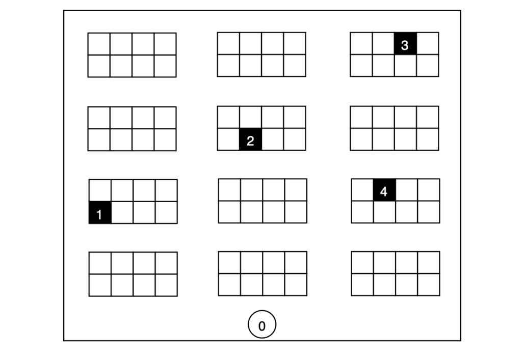
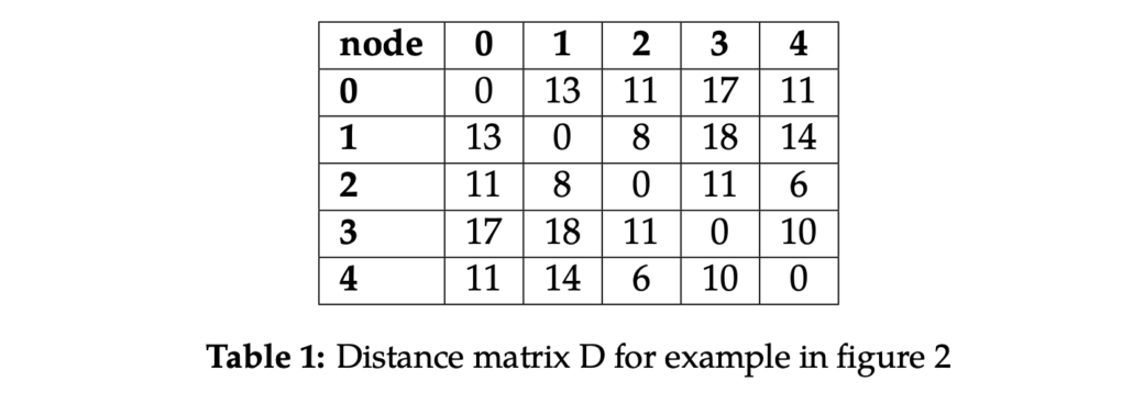
Consider a warehouse organized as shown in figure 2. The agent receives an order requiring the collection of four items from different locations, numbered 1 to 4, starting from location 0. Based on the warehouse design, we can compute the shortest paths between all points and store them in a distance matrix D, sized 5 by 5 (refer to table 1).

Objective  

The agent’s explicit goal is to efficiently visit all pick locations and return to the starting position. For this specific scenario, we can easily calculate the optimal order of node visits by exhaustively considering all permutations, yielding a total of 4! = 24 possibilities. Since the ideal route is known, we can evaluate whether our agent learns the optimal path. In this scenario, the action set remains consistent across all states s ∈ S, thus:

$$A = {0,1,2,3,4}$$

This allows the agent the option to revisit a pick-node that has already been accessed. A state is characterized by a tuple s = (is, Vs), indicating the agent’s current location is and the remaining nodes Vs still unvisited. For instance, s = (2, \{1, 3\}) illustrates the agent positioned at pick-location 2 with outstanding visits to locations 1 and 3. The total set of states can be defined as:

It’s important to verify manually that the total number of states in this example equals 48. More generally, when states are structured this way, the number of states can be calculated as:

In this equation (2), originating from location 0, there are 2^|A|−1 potential combinations of locations remaining to visit; for the other (|A| − 1) locations, 2^|A|−2 possible combinations of still unvisited spots exist. For any given state, the subsequent state resulting from any action is predetermined. For example, if the agent is in state (0, {1, 2, 3, 4}) and chooses to head to pick location 3, the next state becomes (3, {1, 2, 4}). Formally, we define the state-action-transition probability as:

Next, we need to establish the reward function. The agent incurs a negative reward for moving from location x to y, equivalent to the distance between points: −D(x, y). If the agent returns to the starting position having visited all designated points, termed as reaching the terminal state, a significant reward of 100 (or a similarly substantial figure compared to the distances) is awarded. The reward is formally expressed as:

Python Implementation  

import itertools
import pandas as pd
from tabulate import tabulate
import random
from sklearn.metrics import euclidean_distances

# Initialize sample data
# 1 starting point (0), 4 pick positions (1,2,3,4)

D = np.array([[0,13,11,17,11], [13,0,8,18,14], [11,8,0,11,6], [17,18,11,0,10], [11,14,6,10,0]])
# locations = [(5,0), (2,5), (4,5), (6,5), (8,5)]
# D = euclidean_distances(locations)*100
np.fill_diagonal(D, 999)

# Generate action set and pick-node list
Actions = set(range(n))
Nodes = Actions.copy()
Nodes.remove(0)

# Create all potential states
states = []
for j in range(n):
  if j > 0:
    subset = Nodes.copy()
  if j == 0:
    subset = Actions.copy()
  subset.remove(j)
  for i in range(len(subset)+1) :
    a = list(itertools.combinations(subset, i))
    for k in range(len(a)):
      states.append((j, a[k]))

# Establish the state space transition matrix
Transition = np.zeros([len(states), n])
Transition = Transition.astype(int)

for i in range(len(states)):
  for j in range(n):
    new_set = set(states[i][1])
    new_set.discard(j)
    new_set = tuple(new_set)
    state = (j, new_set)
    Transition[i, j] = states.index(state)

# Next, we define the reward matrix with negative distances
Reward = np.zeros([len(states), n])

for i in range(len(states)):
  for j in range(n):
    bonus = (i>0)*(len(state[i][1]) == 0 and j == 0)
    Reward[i, j] = -D[states[i][0], j] + bonus*100

Q-learning Approach  

Multiple reinforcement learning algorithms are available for training the agent, with Q-learning being the most popular, introduced by Chris Watkins in 1989. The algorithm features a function that evaluates the quality of each action-state combination:

$$Q:S×A→R$$

The Q-value Q(st, at) roughly indicates how effective an action at is when the agent is in state st. Q-learning updates the Q-values iteratively to derive the final Q-table filled with Q-values. The agent’s policy can be discerned from this Q-table by selecting the action at in each state st that leads to the highest Q-value. The update rule is as follows:

The algorithm works with these parameters:

• Initial values (Q0): Typically, initial Q-values are set to 0. However, to promote exploration—a concept further explained below—higher initial Q-values may be beneficial, termed as optimistic initial values.
• Learning rate (α): Determines the extent of learning; a rate of 0 means no learning occurs, while 1 means only the latest information is considered.
• Discount factor (γ): Indicates how much emphasis the agent places on future rewards; if γ = 0, only current rewards are weighed.

An episode concludes when the agent reaches a terminal state.

Following a greedy policy means consistently choosing the action yielding the highest Q-value in a given state. Yet, sticking solely to greedy actions can trap the agent in local optima. Thus, we distinguish exploitation from exploration:

• Exploitation: Choosing the action that promises the highest known reward at every iteration.
• Exploration: Opting for an action that may not guarantee the best known reward, providing broader insight into the environment. This could involve random actions or those chosen via a probability function.

One way to balance exploitation and exploration is through ε-greedy strategies. With a probability of 1 − ε, the agent opts for the action believed to provide the best long-term outcomes (exploitation), while with a probability of ε, it randomly selects an action (exploration). Generally, ε remains constant, yet it can be adjusted over time to encourage more exploration during early training phases.

# *** Q-Learning ***
Q_table = np.ones([len(states), n])*1000

# Hyperparameters
alpha = 0.2
gamma = 0.9
epsilon = 0.3

# The algorithm
for i in range (400000):
  begin_state = (0, tuple(Nodes))
  state = states.index(begin_state)
  done = False

  while not done:
    if random.uniform(0, 1) < epsilon:
      action = random.randrange(n) # Explore action space
    else:
      action = np.argmax(Q_table[state]) # Exploit learned values

    next_state = Transition[state, action]
    reward = Reward[state, action]

    if state == states.index((0, ())):
      done = True

    old_value = Q_table[state, action]

    next_max = пр.max(Q_table[next_state])

    new_value = (1 - alpha) * old_value + alpha * (reward + gamma * next_max)
    Q_table[state, action] = new_value

    state = next_state

q_df = pd.DataFrame(Q_table)
q_df.index = states

Next, we will implement this algorithm in Python to resolve our simple order-pick routing scenario. Given the episodic nature with a terminal state, we set the discount rate at γ = 0.9, the learning rate at α = 0.2, and the exploration rate at ε = 0.3.

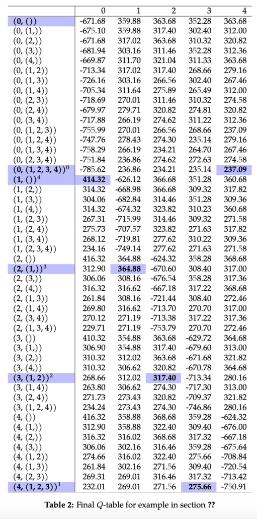
The algorithm runs until the Q-values reach convergence, leading us to the final Q-table shown in table 2. By selecting actions with the highest corresponding Q-values and following the state-action-transition probabilities, the path determined is: 0 → 4 → 3 → 2 → 1 → 0. This indicates the agent visited each pick node once before returning to the starting location, successfully identifying the optimal solution!

Conclusion  

In this post, we provided an introduction to Reinforcement Learning and demonstrated how Q-learning can resolve a basic order-pick routing scenario in a warehouse. However, tackling larger routing scenarios can lead to an explosion in the state space, making Q-table computations impractical. To navigate this challenge, neural networks may be employed to approximate Q-values, eliminating the need for a Q-table for every action-state pair.